
About Me
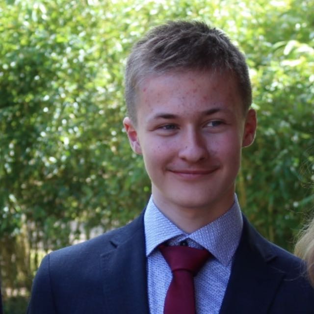
Hi, I'm Adrian.
I like building things.
I've been programming for ten years. I wrote my first program when I was six, and I've been doing it ever since. What fascinates me is how much can come from a simple idea. A few lines of code can become a system, a sketch can become a world, and sometimes an idea that initially sounds ridiculous turns into something worth spending weeks on.
I still enjoy that process as much as I did back then.
I like difficult problems. Mathematics has always been a big part of that, whether it's working on simulations, algorithms, or the formula encyclopedias behind projects like Wave Tracing, Water-Sim, RAPTOR, Cloud, and VELA. Through mathematical competitions, I've learned that not every problem has an obvious solution. Sometimes you just have to try things, get them wrong, and approach them from a completely different direction.
I actually enjoy that.
You'll find projects like RAPTOR, PySpotLite, ARVI, and AirForce Revolution here. They all started with different questions, experiments, or ideas I wanted to explore. Some turned out great. Others taught me what not to do. Both are useful.
Beyond Programming
Code isn't the only thing I like creating. I'm also interested in filmmaking and everything that goes into producing a film.
I've already produced one film, and I'm currently working on a much more ambitious production for our school's Abiball. It's a project involving around 30 people, and I'm involved in pretty much everything: planning, developing ideas, putting together the team, coordinating departments, and making sure all the individual pieces eventually come together.
One thing I've noticed is that I particularly enjoy working with people and building teams. Finding people with different strengths, giving everyone something meaningful to contribute, and watching an idea slowly become a real production is something I genuinely enjoy.
The same goes for other projects. I programmed our school newspaper's website, Lichtblick, which I'm now using to help finance our Abiball through advertising partnerships with companies. It's a good example of how different interests can come together in one project: programming, organisation, and a bit of business.
How I Like to Work
I like working with people who are curious, honest, and willing to question things. I don't think the best projects come from one person having all the answers. They come from people sharing ideas, challenging each other, and occasionally realising that someone else's approach is actually much better.
My experience working with teams at Qestit GmbH and Vogt + Partner GbR has taught me a lot about communication, responsibility, and getting things done even when plans don't go quite as expected.
I care about the technical details, but I also like keeping an eye on the bigger picture. I want to understand how things work, why certain decisions are made, and what could be done better.
What's Next?
I'm interested in software, game development, filmmaking, and the business side of creating things. They might seem like different fields, but to me, they have quite a lot in common.
I don't have everything figured out. I'm still learning, experimenting, and probably starting more projects than I should.
But I've been doing this since I was six, and I don't think I'll run out of things to be curious about anytime soon.
Have a look around. These projects are probably the best way to get to know me.
Projects
Click a project to see details, tech, and visuals.
Categories
Cover
AirForce Revolution
Story Games | Narrative Design
AirForce Revolution
Python
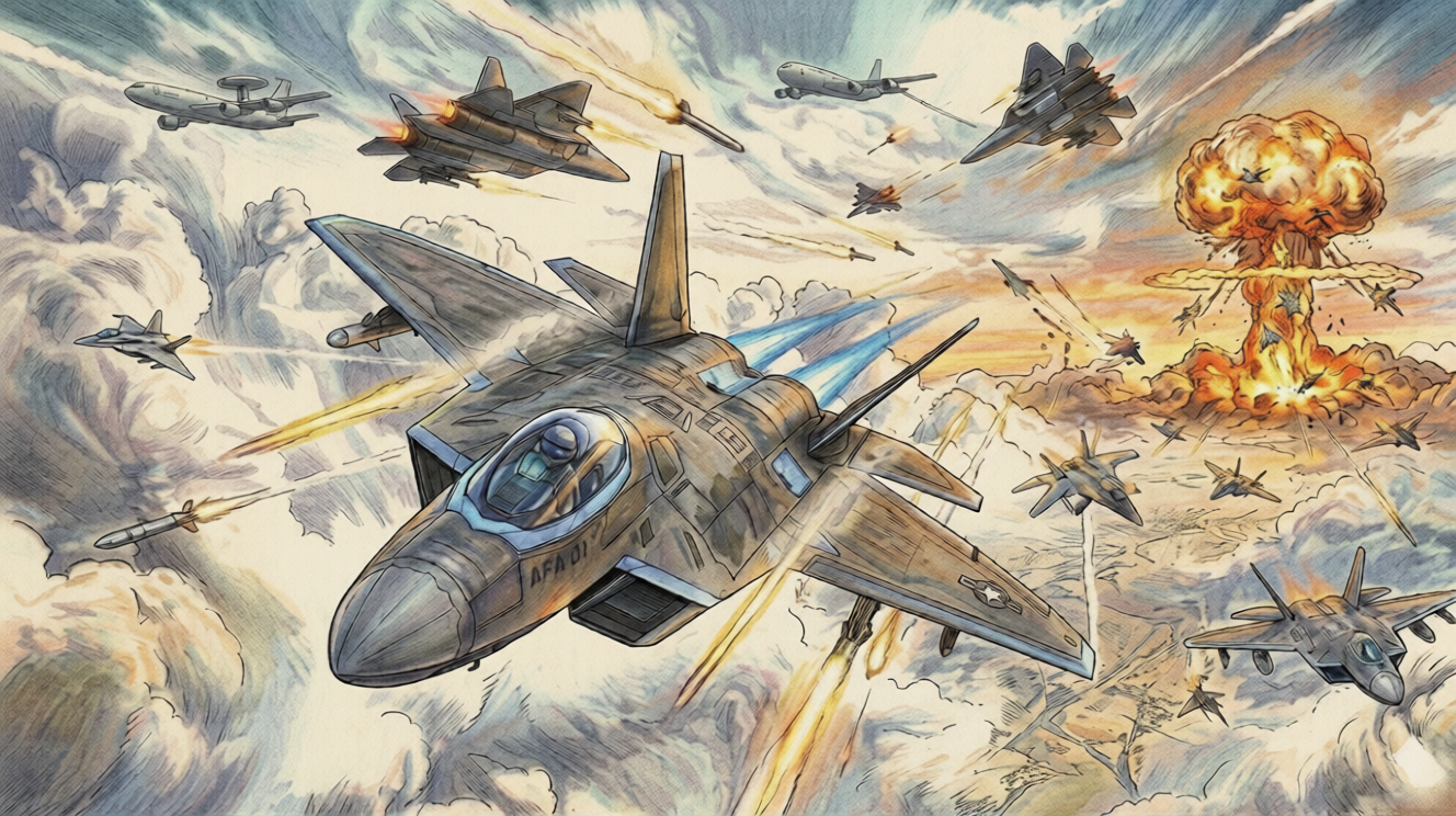
This is a focused excerpt of the game that showcases the algorithmic combat logic. The original project was developed in Python, while this web version was rewritten in JavaScript. Development began in a programming club, but was never completed because the group disbanded. I continued to pursue the project; concept art and live flight calculations are available below.
How a pass is scored
Degrees → Radians
All angle calculations in the game are performed internally in degrees, but are converted to radians for trigonometric functions.
- $\theta_{deg}$: Angle in degrees
- $\theta_{rad}$: Angle in radians (for
Math.sin/Math.cos)
Plane movement (per frame)
The plane moves along its current direction every frame. The angle 0° points upwards; positive angles rotate clockwise.
- $\theta_{rad}$: Current flight angle in radians
- $v_{eff}$: Effective speed (after depth scaling, see Chapter 3)
- $x, y$: Position of the plane in canvas pixels
Speed vector (frame difference)
Is calculated after each position update and used for target prediction.
- $v_x, v_y$: Speed in pixels per frame
- $x_{alt}, y_{alt}$: Position of the previous frame (
lastX,lastY)
Projectile direction vector (when firing)
When firing, the angle is converted into a normalized direction vector, which is then applied to each frame. Frame is applied.
- $d_x, d_y$: Normalized direction vector of the projectile
- $v_{bullet}$: Projectile speed (3,5 – 3,8 px/Frame depending on the team)
Scaling factor from depth
Planes can be at different heights (Z-levels 0–3). The higher the Z-offset, the smaller and slower the object appears – a simple perspective simulation.
- $s$:
scaleFactor∈ (0, 1] - $z$:
zOffset, integer 0 – 3 - At $z=0$: $s=1{,}0$; at $z=3$: $s \approx 0{,}455$
Effective speed
The actual distance traveled per frame scales proportionally to the scaling factor – further distant planes move seemingly slower.
- $v_{base}$: Base speed of the plane (2,2 – 2,4 px/Frame)
- $s$: Scaling factor (see above)
Smooth Z-Offset interpolation (per frame)
Switching between height levels does not happen immediately, but stepwise with a fixed rate of 0,03 per Frame.
- $z_{ziel}$: Target Z-Offset (integer 0–3)
- $z_t$: Current (continuous) Z-Offset of this frame
Target prediction (Lead Shooting)
The AI does not shoot at the current position of the target, but at its predicted position in 18 frames.
- $x_{pred}, y_{pred}$: Predicted target position
- $v_{x,ziel}, v_{y,ziel}$: Speed vector of the target (from Chapter 2)
- $18$: Lead-Time in Frames
Target angle to predicted position
Calculates the angle the plane must turn to aim at the predicted target position.
- $\theta_{ziel}$: Target angle in degrees (0° = up, 90° = right)
- $\mathrm{atan2}(y, x)$: Arcsine with quadrant recognition
Shortest angle difference
Determines the shortest turning path between the current and target angle (always in the range −180° to +180°), to handle both left and right turns correctly.
- $\delta\theta$: Shortest turning direction and size in degrees
- Positive = clockwise, negative = counterclockwise
Rotation rate limiting (Clamping)
The AI turns at most at a mode-dependent rotation rate per frame – scaled with depth, so that distant distant planes do not appear too agile.
- $\omega$: Maximum rotation rate in degrees/frame (mode-dependent, see Chapter 5)
- $s$: Scaling factor from Chapter 3
Avoidance angle (Collision avoidance)
When two planes are approaching each other at less than 200 px, each calculates an avoidance course – exactly the opposite direction of the other.
- $\Delta x, \Delta y$: Vector from own plane to the other
- $+ 180°$: Reverses the direction (flies away from the other)
- Maximum rotation rate here: $\omega_{avoid} = 3{,}8 \cdot s$ (°/Frame)
Scaled rotation rates by mode
All rotation rates are multiplied by the scaling factor $s$ so that the control works consistently on all depth levels.
- Pursuit-Standard: Target outside the 16° shot corridor
- Pursuit-Target: Target within 16° angle difference
- Patrol: No active target or neutral state
- Avoidance: Active avoidance maneuver ($\times 5$ per frame, no Clamping)
- Collision: Narrow-range avoidance in case of overlap
Euclidean distance
Basic distance formula for all distance checks in the game (collision, shot range, AI decisions).
- $d$: Distance in canvas pixels
- $\Delta x, \Delta y$: Position difference between two objects
Depth-scaled range
All AI range thresholds are inversely scaled with the scaling factor so that they remain constant in canvas pixels, independent of the flight height.
- $r_{Kollision} = 22$: Collision radius of a plane (
PLANE_COLLISION_RADIUS) - $s$: Scaling factor of the requesting plane
Projectile hit radius
A hit is registered when the distance between the projectile and the target is less than this dynamic radius – larger planes are easier to hit.
- $r_{bullet} = 12$: Base collision radius of the projectile (
BULLET_COLLISION_RADIUS) - $w_{img}$: Width of the target sprite in its original size
- $s$: Scaling factor of the target
Maneuver entrance probabilities (per frame)
Every frame a random value $r \sim U(0,1)$ is drawn. The maneuver starts when $r$ is less than the threshold and all conditions are met.
- At 60 FPS $P=0{,}001$ corresponds to an average waiting time of $\approx 16{,}7$ seconds
- At $P=0{,}005$ ca. $\approx 3{,}3$ seconds average waiting time
- All probabilities only apply when
maneuverTimer ≤ 0
Smoke particles during crash (Bernoulli)
Every frame smoke and spark particles are generated stochastically.
- Each particle appears at a uniform random position in the range $[\text{pos} - 10,\ \text{pos} + 10]$ px
Particle movement (per frame)
Each particle moves with a slightly disturbed speed vector and shrinks continuously.
- $v_x, v_y$: Initial particle speed (set when created)
- $\varepsilon$: Random noise for organic appearance
Particle transparency (linear decrease)
The opacity of a particle decreases linearly with its remaining lifetime.
- $t$: Remaining lifetime (
lifetime) - $t_0$: Original lifetime (
initialLifetime) - $f$: Fade speed (
fadeSpeed, Standard 1) - $\alpha \in [0, 255]$: Opacity for
rgba()
Particle size (linear shrinkage)
The particle size decreases by a fixed amount each frame and cannot become negative.
- $r_t$: Radius of the particle in pixels
- Represented as a filled circle with $\mathrm{arc}(x, y, r, 0, 2\pi)$
Random offset per frame
As long as the shake duration is active, the origin of the canvas transformation is shifted by a random offset each frame.
- $I$: Current intensity (
cameraShakeIntensity) - On hit: $I = 2$, Duration $= 5$ Frames
- On explosion: $I = 10$, Duration $= 15$ Frames
- Multiple hits: $I = \max(I_{alt}, I_{neu})$ – strongest value wins
Canvas aspect ratio (16:9)
The canvas height is always derived from the width to enforce the aspect ratio.
- $w$: Canvas width in logical pixels
- $h$: Canvas height in logical pixels
Device-Pixel-Ratio (DPR) scaling
On high-resolution displays (Retina) physical canvas pixels are multiplied by the DPR, while the logical context is scaled back.
- $dpr$:
window.devicePixelRatio(typically 1 or 2) - Result: 1 logical pixel = $dpr$ physical pixels (sharp display)
Wrap-Around-Margin (Screen edges)
Planes that leave the screen appear on the opposite side. The margin prevents the sprite from being cut off when it crosses the screen.
- $m$: Wrap-Around-Margin in pixels
- $w_{sprite}$: Original sprite width in pixels
- $s$: Scaling factor of the plane
Sprite scaling when drawing
Each object is scaled and centered at its position when drawn.
- Drawn after
ctx.translate(x, y)andctx.rotate(θ) - Offset $-w/2$, $-h/2$ centers the sprite at the rotation point
Star brightness animation (Ping-Pong)
Each star has a brightness that oscillates between 100 and 255. When the range is left, the direction reverses.
- $B \in [0, 255]$: Brightness (used for RGB-grayscale)
- $\delta \in \{-1, +1\}$: Animation direction
Health ratio (Health Bar)
Determines which portion of the health bar is filled, and is used for the visual display in the HUD.
- $HP_{max} = 5$: Maximum hit points of each plane
- Bar total width: 60 px, height: 6 px
Motor frequency and volume
The pitch and volume of the engine scale linearly with the speed intensity of the plane.
- $I \in [0, 1]$: Normalized speed intensity (
speedFactor) - $f$: Oscillator frequency in Hz (68 Hz at idle, 160 Hz at full speed)
- $G$: Gain value of the audio node
Speed doubling during boost
When a boost maneuver is activated, the current speed is immediately doubled; after the maneuver duration, it returns to the base speed.
- $v_{base}$: Base speed before the maneuver
- Boost duration: $\mathcal{U}(60, 120)$ Frames
- After the duration: $v \leftarrow v_{base}$
Tumbling & falling during crash
A shot plane rotates with a fixed angular velocity and falls downwards while tumbling sideways.
- $\omega_{crash}$: Rotational speed during crash (randomly left or right)
- Crash duration: $\mathcal{U}(60, 120)$ Frames, then explosion
- Speed during crash: $v_{base} \cdot 0{,}5$ (halbiert)
Easing-Funktion (easeInOutCubic)
Used for the smooth scrolling of the navigation links – accelerates at the beginning and slows down at the end.
- $t \in [0, 1]$: Normalized progress of the animation
- Animation duration: $\mathrm{clamp}(|d|, 600, 1400)$ ms, where $d$ = Scroll distance in pixels
With gratitude
ARVI
Python JavaScript HTML CSS
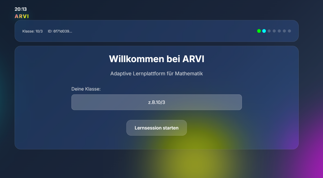
I developed a full web-based learning platform in Python using Flask that guides students step by step through sine theorem exercises. The system manages user sessions, records every answer, tracks time spent, and calculates accuracy. I also integrated AI tools: CLUE provides guided hints, while CORA grades responses and delivers feedback. At the end of each session, the platform generates personalized feedback.
Page 1
Login screen
Select a page, browse screenshots, click the image to zoom.
PySpotLite
Python
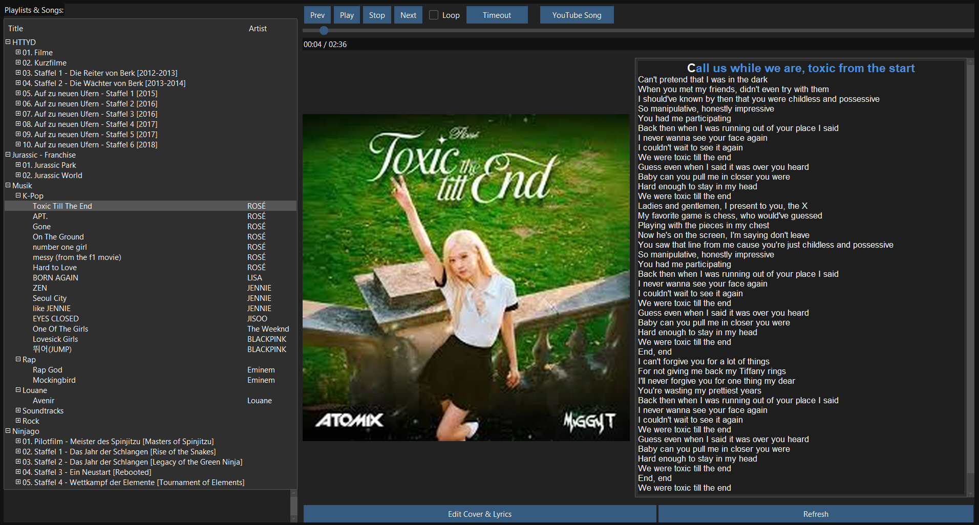
PySpotLite is a local music player that organizes playlists and folders, plays tracks via VLC, displays and manages cover art and lyrics, imports local MP3s, and downloads audio from YouTube. The app features AI-assisted lyric generation and verification using Whisper and Gemini, as well as timeout and song limit controls. During downloads, PySpotLite automatically fetches cover art, identifies the original artist, and can generate time-coded lyrics for live display.
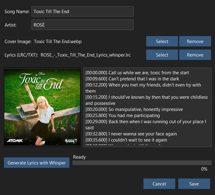
Click an image to enlarge it.
What the light is doing
LRC-Timestamp → milliseconds
Converts an LRC timestamp in the format [mm:ss.xx] into absolute milliseconds, as they are used internally for lyrics matching.
- $\text{min}$: Share of minutes from the LRC tag, $\text{min} \in \mathbb{N}_0$
- $\text{sec}$: Share of seconds from the LRC tag, $0 \leq \text{sec} \lt 60$
- $\text{ms}$: Share of milliseconds — Decimal places $\times\, 100$
- $t_{ms}$: Absolute timestamp in $\text{ms}$, directly comparable to VLC output
Seconds → Minutes & Remaining Seconds (Floor Division)
Splits a total time into minutes and seconds for display in MM:SS format.
- $t$: Total time in seconds as a $\text{float}$, e.g., $t = 133.7\,\text{s}$
- $\text{min}$: Integer minutes — Python: $\lfloor t / 60 \rfloor$
- $\text{sec}$: Remaining seconds — Python: $t \bmod 60$, always $0 \leq \text{sec} \lt 60$
Centiseconds from Fractional Part
Extracts hundredths of a second (centiseconds) from a floating-point number for the LRC format ([mm:ss.cs]).
- $t$: Time in seconds as a $\text{float}$, e.g., $t = 73.42\,\text{s}$
- $\lfloor t \rfloor$: Integer part — Python: $\texttt{int}(t)$
- $cs$: Centiseconds, integer, $0 \leq cs \leq 99$
Milliseconds → Seconds
Converts the audio duration in milliseconds provided by pydub/VLC into seconds.
- $t_{ms}$: Audio duration in milliseconds (e.g., returned by
len(audio)) - $t_s$: Duration in seconds
Total Time → Days / Hours / Minutes / Seconds
Splits an arbitrarily long total duration into days, hours, minutes, and seconds for batch display.
- $T$: Total duration in full seconds
- $d$: Days (86400 = 60 × 60 × 24)
- $h$: Hours (0–23)
- $m$: Minutes (0–59)
- $s$: Seconds (0–59)
Required Amplification (Gain)
Calculates how much amplification is needed to bring an audio clip to the target level. The calculated value is clamped to 0–30 dB to avoid distortion.
- $\text{dBFS}_{target}$: Target level, here −10.0 dBFS
- $\text{dBFS}_{current}$: Current level of the audio clip (pydub:
audio.dBFS) - $G_{clamped}$: Gain to be applied in dB
Normalization with Headroom
Normalizes the loudest sample to 0 dBFS minus a safety margin (headroom) to prevent clipping.
- $H$: Headroom in dB, here 3.0 dB (Call:
audio.normalize(headroom=3.0)) - $\text{PeakLevel}_{max}$: Resulting maximum level = −3.0 dBFS
Dynamic Compression Parameters
Calls the compressor to boost quiet passages and attenuate loud ones – improves speech intelligibility for Whisper transcription.
- $T$: Threshold = −20.0 dBFS (Activation threshold)
- $R$: Ratio = 4:1 (Compression ratio)
- $\text{Attack}$: 5 ms (Attack time)
- $\text{Release}$: 50 ms (Release time)
- $x$: Input level in dBFS
Slider Position → Playback Time
Converts the percentage value of the seek bar (0–100) into an absolute time position where the player should jump to.
- $v$: Slider value (0–100)
- $L$: Total length of the track in milliseconds
- $t_{seek}$: Target time position in milliseconds
Playback Position → Slider Value
Updates the seek bar based on the current playback position — the inverse formula of the above.
- $t_{current}$: Current playback position in seconds
- $t_{total}$: Total length in seconds
- $v$: Slider percentage value to display (0–100)
Visible Share & Scroll Target Position
Calculates how much of the lyrics text box is visible and constrains the scroll position so that the active text block is always within the visible area.
- $h_{text}$: Pixel height of the visible text widget
- $n_{lines}$: Total number of text lines
- $h_{line}$: Pixel height of a single text line
- $f_{visible}$: Visible share (0–1)
- $y_{raw}$: Raw target position of the active line (relative, 0–1)
- $y_{target}$: Constrained scroll position for
text.yview_moveto()
Smooth Scroll Progress
Generates a normalized progress value between 0 and 1 at each animation step for smooth scrolling.
- $i$: Current animation step (0-based)
- $N_{steps}$: Total number of steps
- $p$: Normalized progress value
Batch Percentage Value
Calculates the progress as a percentage during batch lyrics generation.
- $i$: Number of songs already processed
- $N$: Total number of songs to process
- $p\%$: Percentage progress (0–100)
Whisper Time Estimation
Estimates the remaining processing time based on elapsed time and current progress. A safety factor of 1.2 compensates for overhead.
- $t_{audio}$: Length of the audio clip in seconds
- $T_{est}$: Estimated total processing time (incl. 20% overhead)
- $t_{elapsed}$: Time elapsed so far in seconds
- $p_{target}$: Planned phase percentage value
- $p_{cur}$: Currently displayed percentage value
- $t_{remaining}$: Estimated remaining time in seconds
Batch Time Estimation (Whisper Factor)
Adds up the duration of each song, weighted by an empirically determined Whisper factor, to predict the total processing time.
- $d_i$: Duration of the i-th song in seconds
- $0.6208$: Empirical Whisper time factor (processing time / audio duration)
- $T_{batch}$: Total estimated processing time in seconds
Available RAM in Gigabytes
Reads the free RAM in bytes and converts it to gigabytes to select the optimal Whisper model size.
- $\text{available\_bytes}$: Free RAM in bytes (from
psutil.virtual_memory().available) - $1024^3$: Bytes per gibibyte
- $\text{RAM}_{GB}$: Available memory in GB → Model selection: >4 GB = base, >2 GB = small, otherwise tiny
Text Centering on Image (Overlay)
Calculates the top-left corner of a text so that it is rendered centrally within the image.
- $W, H$: Width and height of the target image in pixels
- $w, h$: Width and height of the rendered text in pixels
- $x, y$: Pixel coordinate of the top-left corner of the text block
Blank Line Pattern After Every 4 Lyrics Lines
Inserts a blank line after every fourth content-based lyrics line to improve readability. The condition uses modulo on the offset line index.
- $i$: Current line index in the
lrc_linesarray (0-based) - $4$: Offset to skip the header lines (ti, ar, al, by, …)
- A blank line is inserted if the condition applies and the line is not a header tag
Playlist Navigation: Circular Index
Switches to the next folder/playlist in a list and automatically jumps back to the first element at the end – a classic ring buffer.
- $i_{current}$: Current index in the folder list
- $N$: Total number of folders
- $i_{next}$: Index of the next element (wraps around)
RAPTOR
CSS HTML JavaScript TypeScript
1,500 Neural Minds. Infinite Evolution. Welcome to survival of the fastest, R.A.P.T.O.R.
R.A.P.T.O.R. is an interactive sandbox in which hundreds of digital vehicles learn to drive completely autonomously, without external libraries.
True Evolution: Through neural networks (7→10→8→2 architecture) and genetic algorithms, the genes of the best drivers are combined, while unsuitable ones are eliminated.
Real-time Sensing: Each car autonomously scans its surroundings using 5-channel laser radar (Lidar) and calculates edge collisions down to the pixel.
God Mode: Draw new obstacles in the path with a mouse click and force the AI to adapt to changing conditions in real time, in a fraction of a second.
Don’t just watch code being written, watch it optimize itself!
Xavier Weight Initialization
When creating the network, all weights are randomly initialized using the Xavier method. The goal is to maintain a stable variance of activations across layers and avoid the vanishing/exploding gradient problem.
- wij: Weight from neuron j to neuron i
- 𝒰(−1, 1): Uniformly distributed random number in the interval [−1, 1]
- nin: Number of inputs to the current layer (fan-in)
Weighted Sum of a Neuron
Forward Propagation: Each neuron calculates the weighted sum of its inputs plus bias. This is the core operation of every fully connected layer.
- zj(l): Pre-activation value of neuron j in layer l
- bj(l): Bias of neuron j in layer l
- wjk(l): Weight between neuron k (layer l−1) and neuron j (layer l)
- ak(l−1): Activation of neuron k from the previous layer
- nin: Number of neurons in the previous layer
ReLU Activation Function (Hidden Layers)
All hidden layers use the Rectified Linear Unit (ReLU). It suppresses negative pre-activations and sets them to 0, which promotes sparsity and enables fast learning.
- aj(l): Activation (output) of neuron j in layer l
- zj(l): Pre-activation value (weighted sum + bias)
Tanh Activation Function (Output Layer)
The output layer uses the hyperbolic tangent to bound the network outputs to the interval [−1, 1]. This allows the network to map directly onto normalized control signals (acceleration and rotation).
- aj(L): Output of neuron j of the final layer L
- zj(L): Pre-activation value in the output layer
- Output[0] ∈ [−1,1]: Controls acceleration
- Output[1] ∈ [−1,1]: Controls rotation
Sensor Angle
Each car has 5 sensors arranged in a fan-like pattern around the driving direction. The angle of the i-th sensor is calculated relative to the current vehicle orientation.
- θi: Absolute angle of the i-th sensor (radians)
- θ_{\text{car}}: Current heading of the car (radians)
- i: Index of the sensor (0 to n−1)
- n = 5: Total number of sensors
- π/4 = 45°: Angular spacing between adjacent sensors
Sensor Endpoint (Cartesian Projection)
The maximum endpoint of each sensor is determined by polar coordinate conversion. From this point outward, intersections with obstacles are checked.
- xcar, ycar: Current position of the car
- θi: Angle of the i-th sensor
- Ls = 200: Maximum sensor length in pixels
Sensor Normalization
The measured raw distance is mapped to a normalized value between 0 and 1, which serves as input for the neural network. A value close to 1 means an obstacle is very near; 0 means the line of sight is clear up to the maximum range.
- ri ∈ [0, 1]: Normalized sensor value (input to NN)
- di: Measured distance to the nearest obstacle
- Ls = 200: Maximum sensor length (normalization factor)
Ray-Edge Intersection (Distance to Canvas Border)
The distance from a sensor ray to a canvas edge is computed via ray parameter t. For each of the four edges, it checks when the ray intersects it; the minimum of all positive t-values yields the actual distance.
- dx = cos(θi), dy = sin(θi): Direction vector of the ray
- W, H: Canvas width and height in pixels
- t: Ray parameter (dimensionless)
- dborder: Resulting distance to the closest hit edge
Line-Line Intersection (Sensor ↔ Obstacle Edge)
For each of the 4 edges of a rectangular obstacle, it checks whether the sensor ray intersects that edge. To do this, barycentric parameters t and u are calculated. An intersection exists if and only if both parameters lie within [0, 1].
- (x1,y1)–(x2,y2): Sensor ray (car position → sensor end)
- (x3,y3)–(x4,y4): An edge of the obstacle rectangle
- Δ: Determinant (≈ 0 → parallel lines, no intersection)
- t ∈ [0,1]: Position of the intersection on the sensor ray
- u ∈ [0,1]: Position of the intersection on the obstacle edge
Velocity Update
The acceleration output of the neural network is scaled and added to the current velocity. The factor 0.2 acts as an inertial damping element.
- vt: Current velocity in pixels/frame
- out0 ∈ [−1, 1]: Acceleration output of the NN (Tanh)
- 0.2: Scaling factor (inertia constant)
Velocity Limiting (Clamp)
Following the update, velocity is restricted to a physically realistic interval. Reversing is allowed but limited to half of the maximum forward velocity.
- vmax = 5: Maximum forward velocity [px/frame]
- −vmax/2 = −2.5: Maximum backward velocity
Angle Update (Rotation)
The second output neuron controls steering. The rotation speed is determined directly by the scaled network output and added to the vehicle's heading angle.
- ω: Rotational velocity [rad/frame]
- out1 ∈ [−1, 1]: Rotation output of the NN
- ωmax = 0.1: Maximum rotational velocity [rad/frame]
- θt: Current heading angle of the vehicle [radians]
Position Update (Equation of Motion)
The new position of the vehicle is computed by integrating the velocity along the driving heading — classic kinematic Euler integration in Cartesian coordinates.
- xt, yt: Current position [px]
- θt+1: Updated vehicle angle
- vclamp: Clamped velocity
Traveled Distance (Euclidean)
The straight-line distance between the starting and current position is used as a performance indicator and factored into the fitness function.
- (x, y): Current position
- (x0, y0): Starting position of the vehicle
- d: Euclidean distance to the starting point [px]
Fitness Function
Fitness evaluates an individual's overall performance as a weighted sum of distance, survival time, and speed. A bonus rewards exceptionally long-lived individuals.
- F: Fitness value of the individual
- d: Traveled Euclidean distance
- t: Survival time in frames (timeAlive)
- |v|: Absolute value of the current velocity
- B: Survival bonus (100 points when t > 500 frames)
AABB Collision Detection
For each obstacle, it checks whether the vehicle (modeled as a point + width/height) overlaps the bounding box of the obstacle — Axis-Aligned Bounding Box (AABB) test.
- (x, y): Position of the vehicle (top-left corner)
- wc = 20, hc = 10: Width and height of the vehicle [px]
- (xh, yh): Position of the obstacle
- wh, hh: Width and height of the obstacle
Average Population Fitness
The arithmetic mean of all fitness values in a generation serves as a convergence indicator and a metric for the overall progress of the population.
- F̄: Average fitness of the population
- N: Population size (= 200)
- Fi: Fitness of the i-th individual
Tournament Selection
In tournament selection, k random individuals are sampled from the population. The individual with the highest fitness among these k candidates is chosen as a parent.
- 𝒯: Randomly drawn tournament set (without replacement in expected value)
- k = 5: Tournament size (tournamentSize)
- jl: Randomly chosen index from the population
- Pselection: Selected parent individual (best in the tournament)
Crossover (Recombination)
With probability pc, two parents are combined; each weight and bias has a 50% chance of being inherited from either parent (Uniform Crossover). Otherwise, parent 1 is copied unchanged.
- wij(1,2): Weight of parent 1 and parent 2 respectively
- pc = 0.7: Crossover probability
- 𝒰(0,1): Uniformly distributed random number for each individual weight
Mutational Perturbation
Following crossover, each weight and bias is modified with probability pm by a uniformly distributed random disturbance. This prevents premature convergence and preserves population diversity.
- w'ij: Mutated weight
- pm = 0.1: Mutation probability per weight (mutationRate)
- σm = 0.2: Mutation strength (mutationStrength)
- 𝒰(−1, 1): Uniformly distributed perturbation scaled by σm
VELA
HTML JavaScript GLSL WebGL
Just drag your windows together on your screen to watch glowing orbs fuse and flow like ink in water.
The molecule step
Window identifier token
Each window receives a short unique identifier by encoding a uniform random number in base 36 and taking seven characters.
- u: uniform random number in [0, 1]
- toString36: conversion to an alphanumeric base 36 string
- slice(·, 2, 9): seven characters starting at index 2
Random palette index
At startup, a color is picked at random from a predefined palette by drawing a uniform discrete index.
- i: chosen integer palette index
- N = PALETTE.length: number of colors in the palette
- u: uniform random number
Random HSL color
As an alternative to the fixed palette, a random color is generated in HSL space while keeping saturation and lightness within a vivid, balanced band.
- uk ∼ 𝒰(0,1): three independent uniform samples
- h ∈ [0, 1]: hue, mapped across the full circle
- s ∈ [0.75, 1.00]: saturation kept strong
- l ∈ [0.45, 0.65]: lightness kept in the middle range
HSL helper function h2r
The function h2r is the core of the HSL to RGB conversion. It maps a hue offset t to one RGB channel by piecewise linear interpolation between p and q.
- p, q: intermediate bounds derived from lightness and saturation
- t: hue offset wrapped into [0, 1)
HSL to RGB bounds q and p
Before calling h2r, the upper and lower channel bounds q and p are computed from lightness and saturation.
- l: lightness in [0, 1]
- s: saturation in [0, 1]
- q: upper bound of the RGB range
- p: lower bound of the RGB range
Normalized RGB from hex
A six digit hex color string is converted into three floating point channels in [0, 1] by dividing each byte by 255.
- hex1:3: first two hex digits parsed as an integer for red
- r, g, b ∈ [0, 1]: normalized channel values
Float RGB to hex component
The inverse step rounds a normalized channel value to an eight bit integer before formatting it as two hex digits.
- v ∈ [0, 1]: floating point channel value
- c8bit ∈ {0, …, 255}: eight bit integer channel
Global position with local offset
The screen position of the molecule combines the window center with the simulated local offset. The vertical axis is inverted because canvas coordinates grow downward.
- gcx, gcy: window center coordinates on screen in pixels
- px, py: simulated local offset in pixels
- gx(self), gy(self): resulting global screen position
Stale window filter
Windows that have not sent a heartbeat for more than 1.5 seconds are treated as closed and removed from the simulation.
- tnow: current timestamp in milliseconds
- ti: last known timestamp of window i
- 1500 ms: timeout threshold
Raw window velocity
The unfiltered velocity of the window is the difference in screen coordinates between two consecutive frames.
- xscreen, yscreen: current window position
- xscreenprev, yscreenprev: window position on the previous frame
Exponential velocity smoothing
To damp jitter and sudden jumps from window dragging, the raw velocity passes through a first order low pass filter.
- svx, svy: smoothed window velocity
- α = VSMOOTH: smoothing factor in (0, 1]
Inertial impulse
Window motion pushes the molecule in the opposite direction through an inertia coefficient, so the blob lags and sloshes when the window moves.
- vx, vy: simulated molecule velocity
- svx, svy: smoothed window velocity
- I = INERTIA: inertia strength
Spring force to origin
A linear Hookean spring pulls the molecule continuously back toward the center of its own window.
- px, py: current displacement from the window center
- k = SPRING: spring stiffness
- F = −k·p: restoring force proportional to displacement
Friction damping
At each physics step the velocity is multiplied by a factor below one, simulating viscous drag and keeping the motion stable.
- f = FRICTION: damping factor in (0, 1)
Position integration
Explicit Euler integration adds the current velocity to the local position once per frame.
- px, py: local displacement position
- vx, vy: current velocity in pixels per frame
Offset norm and radius limit
If the Euclidean length of the offset exceeds the maximum radius Dmax, the vector is rescaled back onto the boundary disk.
- dp: Euclidean norm of the offset
- Dmax = MAX_DISP: maximum allowed offset radius in pixels
Delta time cap
Elapsed time between frames is capped from above so the simulation does not explode after a tab or window has been paused.
- t − tprev: actual elapsed time in seconds
- 0.05 s: upper bound of 50 ms
Molecule radius
The metaball radius scales with the shorter side of the window so the molecule stays well proportioned at any aspect ratio.
- W, H: window width and height in pixels
- R: molecule radius in pixels
- 0.22: scale factor of 22 percent of the shorter side
Contact distance and touch check
Two windows count as touching when the distance between their global molecule positions falls below dtouch, which starts the ink blend.
- dtouch: contact threshold at 185 percent of the molecule radius
- gx(o), gy(o): global screen position of another window o
- 1.85: overlap factor so blending begins slightly before hard contact
Centered UV and local UV
The normalized fragment coordinate vUv is centered and scaled to pixels, then expressed relative to the window's own molecule center.
- vUv ∈ [0,1]²: normalized shader fragment coordinate
- res: resolution vector (W, H) in pixels
- ⊙: componentwise multiplication
- pself: center of the local molecule in pixels
- ulocal: coordinate normalized by the molecule radius
Square root accumulation
Colors are averaged in square root space and squared back, which preserves brightness better than a flat linear RGB average.
- ri, gi, bi: channel values of the i th color
- n: number of colors being mixed
- mr, mg, mb: resulting mixed RGB channels
HSL intermediates from mixed RGB
From the mixed RGB color, the maximum, minimum, chroma, and lightness are computed as inputs for hue and saturation.
- mx: maximum of the three channels
- mn: minimum of the three channels
- d: chroma span
- l: HSL lightness
Piecewise saturation
HSL saturation uses a different denominator above and below midpoint lightness.
- d: chroma
- l: lightness
- s ∈ [0, 1]: resulting HSL saturation
Piecewise hue
Hue is computed from whichever channel dominates and then normalized to the unit interval.
- d: nonzero chroma
- mr, mg, mb: mixed RGB channels
- h ∈ [0, 1]: normalized hue
Saturation boost and lightness bounds
After mixing, saturation is boosted so blends do not turn muddy, and lightness is clamped to a clean middle range.
- 1.5 s + 0.2: linear lift that keeps mixed colors vivid
- l ∈ [0.40, 0.70]: clamped lightness range
HUD color interpolation
The displayed molecule color interpolates linearly between the base color and the mixed target color according to the blend factor β.
- BR,G,B: own base molecule color
- MR,G,B: mixed merge color
- β = inkBlend ∈ [0, 1]: blend factor from pure base to full mix
Merge buildup
While two molecules touch, the blend factor β approaches one exponentially, giving the ink transfer a soft ease in.
- β ∈ [0, 1]: blend factor
- tink: time since contact started in seconds
- 0.30: growth rate
Blend decay on separation
Once contact ends, β decays exponentially and snaps to zero below a small threshold.
- 1.8: decay rate, faster than the buildup
- Δt: frame delta time in seconds
- 10−3: cutoff threshold
Merge color return
After separation, the merge color itself drifts exponentially back toward the molecule's base color so no tint remains.
- f ∈ [0,1]: per frame interpolation factor
- 0.8: return rate
- MR,G,B: merge color pulled back toward BR,G,B
Hash projection for noise
A pseudo random gradient at each lattice point is generated from two dot products followed by a sine fractional hash.
- p ∈ ℝ²: lattice coordinate of the noise grid
- sin(·) · 43758.5453: high frequency scramble
- fract(·): fractional part in [0, 1]
- h ∈ [−1, 1]²: pseudo random gradient vector
Smoothstep in gradient noise
Instead of linear interpolation across a grid cell, a cubic Hermite curve removes visible grid seams.
- f: fractional position inside a grid cell in [0, 1]²
- ⊙: componentwise multiplication
- u: smoothed interpolation weight
fBm accumulation
Several octaves of gradient noise are summed with halved amplitude and rotated, doubled frequency to build an ink and smoke texture.
- v: accumulated fBm value
- a: amplitude of the current octave, halved each step
- gnoise(p): gradient noise sample at position p
- Rp: rotation matrix that breaks axis alignment
- 2.03: frequency multiplier per octave
Smooth minimum
The smooth minimum operator blends two signed distance fields so separate circles merge with a soft liquid bridge.
- a, b: signed distances being combined
- k = 85: smoothing radius
- h ∈ [0,1]: interpolation weight
- −k h(1−h): quadratic fillet term
Weighted color field
At every fragment, the field color is the inverse square distance weighted average of all molecule colors.
- u: current fragment position in pixels
- pi: position of the i th molecule
- wi: inverse square weight
- ε = 0.8: small regularizer that avoids division by zero
- ci: color of the i th molecule
- C: resulting field color at the fragment
Circle SDF and union
A circle's signed distance is distance minus radius. All molecules are folded into a single field with the smooth minimum.
- d < 0: fragment lies inside the combined metaball
- d ≥ 0: fragment lies outside in the glow region
- R: molecule radius
- pself, pi: local and neighboring molecule centers
Wavefront mask and pattern mix
During a merge, an ink wavefront expands from the center outward, starting as tendrils and filling into a solid blob.
- tink: time since the merge began in seconds
- tP ∈ [0,1]: normalized wavefront progress
- tendrils: fBm tendril pattern
- β: global blend factor
- 1.3: gain factor for full coverage
Smoke texture
Domain warping feeds one fBm evaluation into the coordinates of a second fBm, producing a swirling smoke pattern inside the molecule.
- sp: scaled and time drifted UV coordinate
- 0.004: spatial frequency scale
- (0.055 t, 0.038 t): drift velocity over time
- 0.75: domain warp strength
- smoke ∈ [0,1]: warped noise remapped to the unit interval
Color mix with ink overlay
The interior color first mixes the own color toward the target color by β, then lays that ink over the base color through inkMask.
- cmy: own molecule color
- ctarget: target color from all touching neighbors
- β: global blend factor
- inkMask: spatial wavefront mask
- 1.6: coverage gain
Interior highlights and sparkle
Inside the negative SDF region, smoothstep ramps create a soft rim and a bright core, while high noise peaks add small sparkles.
- rim: highlight near the outer edge of the sphere
- core: brighter region toward the center
- spark: sharp highlights from noise peaks above 0.80
- 3.5: exponent that tightens the sparkle peaks
- 0.30 rim: subtle darkening near the boundary
Outer glow and alpha
Outside the metaball, two exponential falloffs form a tight and a wide halo around the boundary, combined with smooth edge anti aliasing.
- aa: edge anti aliasing term
- g1: tight inner glow with decay 0.030
- g2: wide outer glow with decay 0.007
- cfield: weighted field color
- α: final alpha channel
Merge state and render branch conditions
Four boolean conditions drive the merge timer and select between interior shading and outer halo rendering.
- |touching|: number of currently touching neighbor windows
- wasMerging: merge state from the previous frame
- d: signed distance of the combined metaball field
- β < 0.002: threshold below which the ink pattern is skipped
Cloud Shader
GLSL WebGL 2
An endless, vibrant sky, painted with light and shadow. Soft, watercolor-like clouds glide across the screen in an eternal, animated drift, while their edges blur like fresh ink in water. A majestic work of art that conveys a sense of infinite freedom.
But beauty is deceptive: this endless sky does not actually exist.
What appears to be an infinite cosmos is a mathematical illusion generated in real time from absolute nothingness. Every brushstroke, every gentle distortion, and every delicate color transition is an algorithmic illusion, a perfectly staged chaos that comes to life only the moment you look at it.
How a cloud is built
Noise Generation
Perlin Noise (3D)
Generates smooth, continuous noise patterns for natural cloud shapes using gradient interpolation.
- $N(x,y,z)$: Noise value at 3D coordinates
- $g_i$: Random gradient vectors at grid corners
- $d_i$: Distance vectors to grid corners
- $f(w)$: Smoothstep interpolation function: $6w^5 - 15w^4 + 10w^3$
Fractal Brownian Motion (FBM)
Combines multiple noise octaves at different frequencies and amplitudes to create detailed cloud structures.
- $p$: 3D position vector $(x, y, z)$
- $n$: Number of octaves (typically 4-8)
- $A_i$: Amplitude for octave $i$
- $F_i$: Frequency multiplier for octave $i$
- persistence: Amplitude decay factor (typically 0.5)
Cloud Density
Height-Based Density Falloff
Clouds become less dense at higher and lower altitudes, creating natural vertical distribution.
- $D_h(y)$: Density multiplier at height $y$
- $y_{\text{center}}$: Center height of cloud layer
- $\sigma$: Vertical spread parameter (controls cloud thickness)
Final Cloud Density
Combines noise with height falloff and applies threshold to create distinct cloud boundaries.
- $\rho(p)$: Final density at position $p$
- $p_y$: Y-component of position $p$
- threshold: Density cutoff value (0.0 - 1.0)
Ray Marching
Volume Ray Marching
Steps through 3D space accumulating cloud density to render volumetric clouds.
- $C$: Final accumulated cloud color/density
- $r_0$: Ray origin (camera position)
- $d$: Ray direction (normalized)
- $\Delta t$: Step size along ray
- $n$: Number of samples (32-128)
- $T_i$: Transmittance (remaining light energy)
Adaptive Step Size
Optimizes performance by taking larger steps in empty space and smaller steps in dense cloud regions.
- $\Delta t_i$: Step size at sample $i$
- $\Delta t_{\text{min}}$: Minimum step size (dense regions)
- $\Delta t_{\text{max}}$: Maximum step size (empty space)
- $\rho_i$: Density at current sample
Lighting & Scattering
Beer's Law (Light Attenuation)
Models how light intensity decreases as it travels through cloud volume.
- $I$: Transmitted light intensity
- $I_0$: Initial light intensity
- $\sigma_t$: Extinction coefficient (absorption + scattering)
- $d$: Distance traveled through medium
Henyey-Greenstein Phase Function
Describes how light scatters within clouds based on viewing angle relative to light direction.
- $P(\theta, g)$: Probability of light scattering at angle $\theta$
- $\theta$: Angle between view direction and light direction
- $g$: Anisotropy parameter (-1 to 1)
- $g > 0$: Forward scattering (typical for clouds: 0.6-0.8)
- $g = 0$: Isotropic scattering
- $g < 0$: Back scattering
Powder Effect (Silver Lining)
Creates bright edges on clouds where light enters, simulating realistic cloud illumination.
- $P_{\text{powder}}$: Powder effect multiplier
- $\rho$: Local cloud density
Animation & Movement
Cloud Motion
Animates clouds by offsetting noise coordinates over time, creating realistic wind-driven movement.
- $p_{\text{anim}}$: Animated position for noise sampling
- $p$: Static world position
- $\vec{v}$: Wind velocity vector $(v_x, v_y, v_z)$
- $t$: Time elapsed (seconds)
Turbulence (Detail Noise)
Adds small-scale detail and wispy structures using higher-frequency noise with faster movement.
- $\rho_{\text{base}}$: Base cloud density
- $\text{FBM}_{\text{detail}}$: High-frequency detail noise
- $\vec{v}_{\text{turb}}$: Turbulence velocity (typically $2-3 \times$ wind speed)
Water-Sim
GLSL WebGL
One step of the water
Wave Equations
Gerstner Wave (Trochoid)
Creates realistic ocean waves with sharp crests and rounded troughs by displacing vertices in circular motion.
- $(x", y", z')$: Displaced vertex position
- $(x, y, z)$: Original flat surface position
- $A$: Wave amplitude (height)
- $\vec{D}$: Wave direction vector (normalized)
- $Q$: Wave steepness factor (0-1, typically 0.5-0.8)
- $\omega$: Angular frequency (radians/second)
- $k$: Wave number = $2\pi / \lambda$ (wavelength)
- $t$: Time in seconds
Dispersion Relationship
Links wave frequency to wavelength for realistic ocean wave speeds based on water depth.
- $\omega$: Angular frequency
- $g$: Gravitational acceleration (9.81 m/s²)
- $k$: Wave number
- $d$: Water depth
For deep water ($d \gg \lambda$): $\omega \approx \sqrt{g \cdot k}$
For shallow water ($d \ll \lambda$): $\omega \approx k\sqrt{g \cdot d}$
Multiple Wave Superposition
Combines multiple Gerstner waves with different parameters to create complex, natural-looking ocean surfaces.
- $P_{\text{final}}$: Final vertex position after all wave displacements
- $P_0$: Original flat surface position
- $\Delta P_i$: Displacement from wave $i$
- $N$: Number of wave layers (typically 3-8)
- $\phi_i$: Phase offset for wave $i$
Normal Calculation
Analytical Wave Normal
Computes surface normals directly from wave derivatives for accurate lighting without tessellation.
- $\vec{n}$: Surface normal vector
- $\partial y / \partial x$: Rate of height change in X direction
- $\partial y / \partial z$: Rate of height change in Z direction
- $\vec{p}$: Position vector $(x, z)$
Normal Map Perturbation
Adds fine detail to waves using texture-based normal maps for small-scale ripples and foam.
- $\vec{n}_{\text{wave}}$: Base wave normal from geometry
- $\vec{n}_{\text{map}}$: Normal from texture map
- $\vec{n}_{\text{up}}$: Default up vector $(0, 1, 0)$
- strength: Detail intensity (0-1)
Lighting & Appearance
Fresnel Effect (Schlick Approximation)
Models how water reflectivity changes with viewing angle - more reflective at grazing angles.
- $F(\theta)$: Fresnel reflectance
- $F_0$: Reflectance at normal incidence (water: 0.02)
- $\theta$: Angle between view direction and surface normal
Refraction (Snell's Law)
Calculates how light bends when entering water, used for underwater visibility and caustics.
- $n_1$: Index of refraction for air (1.0)
- $n_2$: Index of refraction for water (1.333)
- $\theta_1, \theta_2$: Incident and refracted angles
- $\vec{d}_{\text{in}}$: Incoming ray direction
- $\vec{d}_{\text{refract}}$: Refracted ray direction
Water Color & Depth Attenuation
Simulates how water color changes with depth due to light absorption and scattering.
- $C_{\text{water}}$: Final water color
- $C_{\text{surface}}$: Surface color (light blue)
- $C_{\text{deep}}$: Deep water color (dark blue/green)
- $\sigma$: Extinction coefficient (controls clarity)
- $d$: Water depth
Specular Reflection (Blinn-Phong)
Creates sparkles and glints on water surface from direct light reflections.
- $I_{\text{spec}}$: Specular intensity
- $\vec{n}$: Surface normal
- $\vec{h}$: Half-vector between light and view
- $\vec{l}$: Light direction
- $\vec{v}$: View direction
- $\alpha$: Shininess/glossiness (32-128 for water)
Foam & Whitecaps
Foam Generation (Jacobian)
Detects wave compression areas where foam naturally forms using the Jacobian determinant.
- $J$: Jacobian determinant (1.0 = no compression)
- $\Delta x, \Delta z$: Horizontal wave displacements
- threshold: Foam sensitivity (typically 0.8-0.95)
- When $J < 1$: Waves are compressing (foam appears)
Foam Decay
Foam gradually fades over time after wave compression, creating realistic foam trails.
- $F_t$: Foam intensity at time $t$
- $F_{\text{new}}$: Newly generated foam from Jacobian
- $\lambda$: Decay rate (1-5)
- $\Delta t$: Time step (frame delta)
Performance Optimization
Level of Detail (LOD)
Reduces wave complexity and vertex count for distant water to maintain performance.
- $N_{\text{waves}}(d)$: Number of wave layers at distance $d$
- $N_{\text{min}}$: Minimum waves (1-2)
- $N_{\text{max}}$: Maximum waves (6-8)
- $\beta$: LOD falloff rate
- $d$: Distance from camera
Wave Tracing
C++ CMake
SEPT Acoustic Lab simuliert 2D-Schallwellen in Echtzeit: Wände zeichnen, Quellen platzieren, mit dem Hörer durch den Raum gehen (WASD) und sofort hören, wie Material, Distanz und Atmosphäre den Klang verändern. Physik: FDTD-Wellengleichung, Impedanzreflexion, Kantenbeugung, Luftdämpfung.
Following a wave
Physikalische Grundlage von SEPT Acoustic Lab: 2D-Wellengleichung (FDTD), Schallausbreitung in Luft, Materialwechsel, Beugung an Kanten und Echtzeit-Audio-Synthese am Hörer.
1 · Wellengleichung (2D FDTD)
Diskrete 2D-Wellengleichung mit explizitem Leapfrog-Schema:
\[ u^{n+1}_{i,j} = (2 - \delta)\,u^n_{i,j} - (1-\delta)\,u^{n-1}_{i,j} + r^2 \left( u^n_{i+1,j}+u^n_{i-1,j}+u^n_{i,j+1}+u^n_{i,j-1} - 4u^n_{i,j} \right) \]- $u$ — Schalldruck (normiert) am Gitterpunkt
- $r = c\,\Delta t / \Delta x$ — CFL-Zahl (stabil für $r^2 \lesssim 0.25$ in 2D)
- $\delta$ — lokale Dämpfung (Luft + Material)
2 · Schallgeschwindigkeit in Luft
- $T$ — Temperatur in °C
- $\varphi$ — relative Luftfeuchte (0…1)
3 · Geometrische Streuung & Luftdämpfung
Am Hörer wird jede Quelle mit Streuung und exponentieller Luftabsorption gewichtet:
\[ A(d,f,\varphi) = \frac{T_\text{wall}}{1 + 0{,}09d + 0{,}006d^2}\,\exp\bigl(-\alpha(f,\varphi)\,d\bigr) \]- $d$ — Gitterabstand Quelle → Hörer
- $T_\text{wall}$ — Transmissionsfaktor entlang des Strahls (Material + Kantenbeugung)
- $\alpha$ — frequenz- und feuchteabhängiger Absorptionskoeffizient pro Zelle
4 · Impedanzreflexion an Wänden
Reflexionsanteil an festen Zellen; Rest wird gedämpft weitergeleitet. Typische akustische Impedanz der Luft: $Z_\text{Luft} \approx 413\ \text{Pa·s/m}$.
5 · Kantenbeugung (Huygens-Näherung)
Mit $\lambda_\text{beug} = 0{,}022 \cdot N_\text{kanten}$ — jede durchquerte Materialkante öffnet einen kleinen Beugungspfad.
6 · Sponge-Absorber (Randdämpfung)
Verhindert harte Reflexionen am Simulationsrand ($N_\text{sponge}=10$ Zellen).
7 · Echtzeit-Audio am Hörer
Quellen werden bei 48 kHz als Sinus oder Sample synthetisiert; das FDTD-Feld liefert Raumanteil. Stereo-Panning über horizontale Quellenverschiebung.
Lichtblick
PHP JavaScript HTML CSS
I built Lichtblick for my school: a digital newspaper that students use. After signing in with a class code they get recommended stories, polls and trends, and they can write, vote, and join the editorial work. The live paper stays behind login; the screenshots show the start page as readers see it (featuring placeholder content authored by me during development).

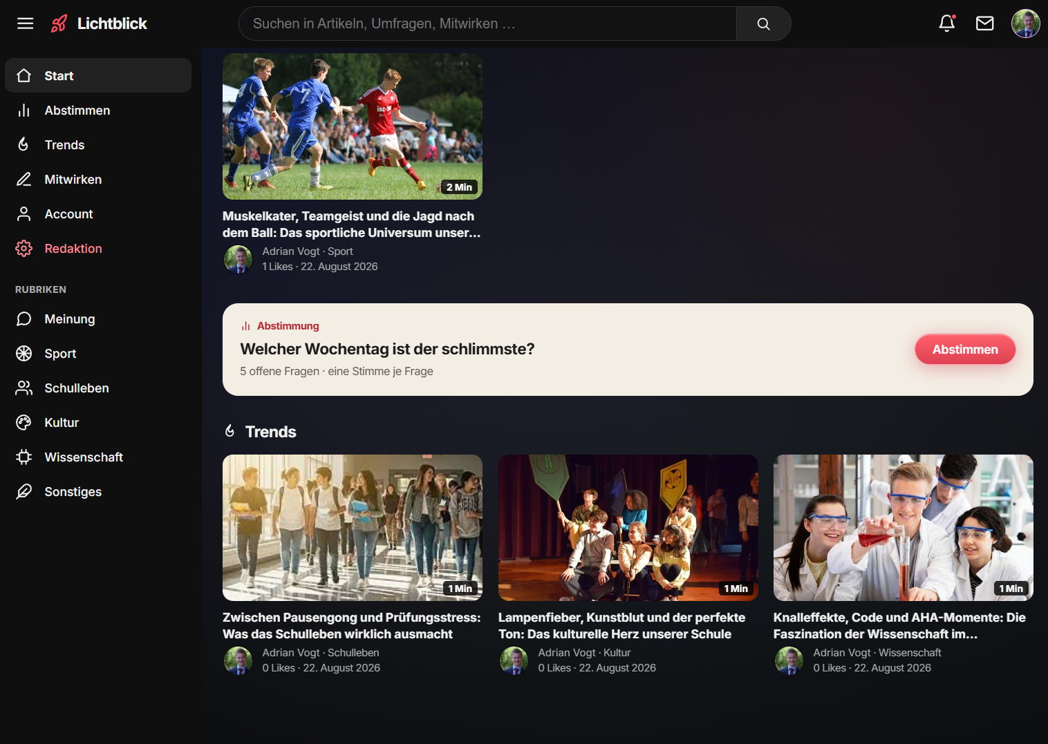
Shyra
HTML CSS JavaScript Python C++ TypeScript XML CMake
This website is the hub for Shyra: project structure, live demos, and technical notes come together in one place. The front end pairs the visual identity with interactive project navigation.
ARVI paper
PDF Mathematics
The scientific paper behind ARVI: traditional mathematics teaching compared with AI-supported learning, written for the platform I built.
Time Superposition
Mathematics Physics
An idea of how the universe might work, inspired by my interest in theoretical physics.